|
|

|
|
|
|
In this project, we implemented a path tracer that can render scenes with triangles and spheres. We also implemented a bounding volume hierarchy(BVH) to accelerate the rendering process by Then in part 3, we simulated light transport in the scene with two different implementations: hemisphere sampling and importance sampling. Next, we further implemented full global illumination by tracking multiple bounces. Finally, we accelerated the rendering process by implementing a adaptive sampling, which concentrating the samples in the more difficult parts of the image.
For the ray generation part, we first generate the camera ray by calculating the position (x,y) on the image plane in terms of view angles, then apply the camera transformation to get the ray direction. Then we use the ray we generated previously to estimate the brightness of the pixel with monte carlo estimation. For each camera ray at that pixel, we incorporate it into the Monte Carlo estimate of the value of the pixel, then normalize the result in the end.
Then we test if the ray intersects with the triangle. If it does, we calculate the intersection point and the normal at that point. Then we use the intersection point and the normal to calculate the color of the pixel. same for sphere.
We used the Moller Trumbore algorithm introduced in class. By definition a point resides inside a triangle can be represented as weighted sums in Barycentric coordinate systems. Then by solving
$\begin{bmatrix} t \\ b1 \\ b2 \end{bmatrix} = \frac{1}{S_1 * E_1} \begin{bmatrix} S_2 * E_2 \\ S_1*S \\ S_2 * D \end{bmatrix} $
where $S_1, S_2, S$ are the cross products of the vectors $E_1, E_2, D$ respectively. Then we can calculate the normal at the intersection point by $N = b1N_1 + b2N_2 + (1-b1-b2)N_3$ (if intersection exists)
|
|
|
|
|
|
I first iterated through the start and end iterables to calculate # of primitives and the average centroid of 3 dimensions. Then I test if the current node is a leaf node. If it is, create a leaf node and return it. If not, the average of centroids heuristics is being used. I first pick the axis with largest extent, and then compare the centroids of different triangles against the average centroid on that axis, partition them info two groups, and recursively call the function to create the left and right child nodes.
I chose the average of centroids heuristics it can almost evenly split the triangles into two groups(in most of the cases), and it is easy to implement. Except for the case where most triangles reside in one side of the plane, then average of centroids will not work very well, but it's hardly the case in practice. The centroids heuristics works well in all the large .dea files provided.(potential extra credit) I also implemented the iteration version of construct_bvh, but it does not work well. From the program output, the number of rays traced by BVH is siginificantly higher, thus the rendering time is longer. Not sure why this is the case so I commented out the code. My implementation is as follows:
I created a stack and a node struct containing 1. stard 2. end 3. parent 4. is_left. I also created a root node and test if the root node is a leaf node. If not, parse it into 2 child nodes, and push them into the stack. For each node popping out of the stack, set parent.l = curr if is_left is true, and parent.r = curr otherwise. The rest is basically the same with the root node. Fianlly when the stack is empty, return the root node (saved with a pointer)

|
|
|
|
My CPU is m1 pro with 16g ram.
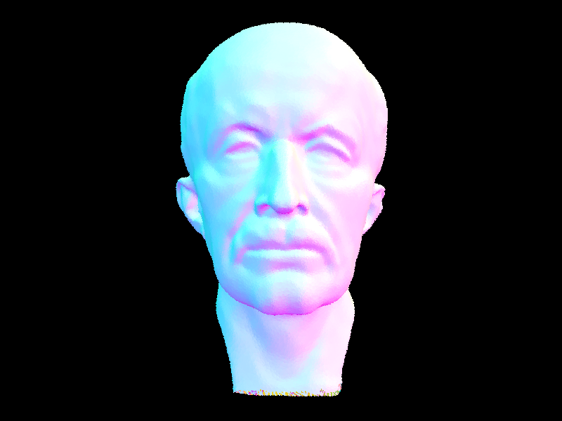
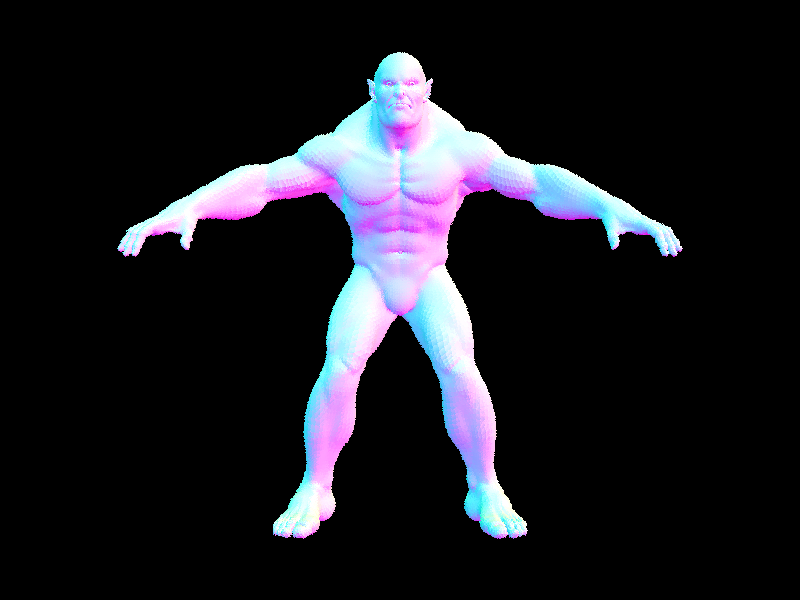
Beast.dae has 64618 triangles and it takes 46.3s to render without BVH, and 0.0358s to render with BVH.
CBlucy.dae has 133796 triangles and it takes 65s to render without BVH, and 0.0448s to render with BVH.
The result above shows that BVH does accelerate the rendering process significantly by reducing the number of calculations needed.
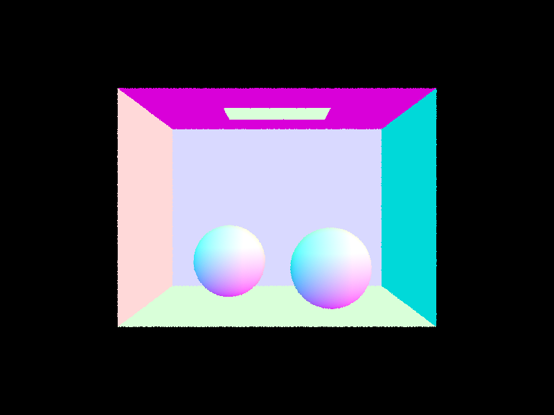
We first implemented the BSDF function, which evaluates diffuse lambertian BSDF.(reflectance / pi), and the zero_bounce_radiance, which evaluates the what lights should look like if there are no bounces at all.
Then we implemented direct lighting with uniform hemisphere sampling. We first iterate through all the sample lights, and for each light, we unfirormly randomly sampled on the hemisphere, and calculate the ray from w_in to hit point intersects with the BVH, if is, we calculate the light contribution with the reflection equation, and add it to the total light contribution.
Finally we implemented direct lighting with importance sampling. Similiar with the uniform hemisphere sampling, we first iterate through the lights in the scene, then if the light source is a single light source, we only sample once. If not, we sample directions between the light source and the hit_p but based on the pdf we created. Then if the ray from w_in to hit point intersects with the BVH, we know the hit point is in shadow and the light does bounce. We calculate the light contribution with the reflection equation, and add it to the total light contribution.
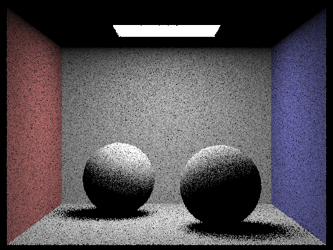
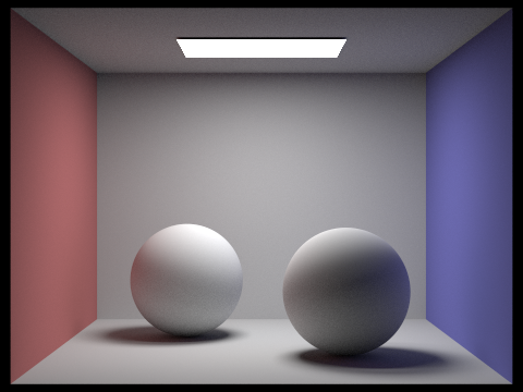
| Uniform Hemisphere Sampling | Light Sampling |
|---|---|
|

|
|
|
|
|

|

|
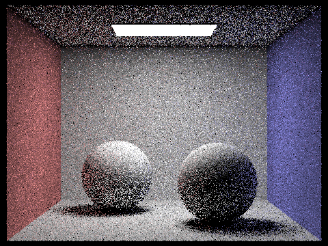
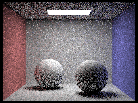
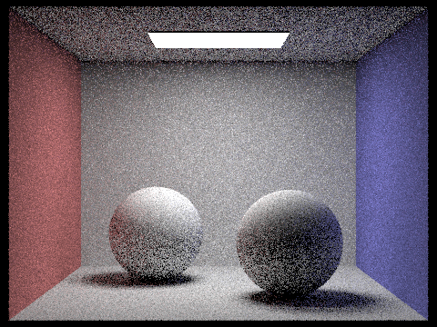
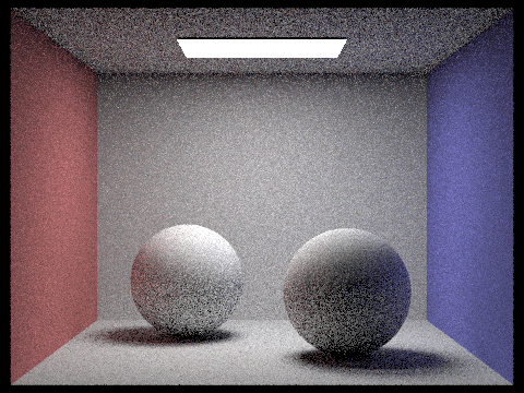
In importance sampling, we estimate the rendering equation by sampling it with a PDF, which means all lights may or may not be sampled . In 1 light ray image above, we can see the noise is obvious, and the reason behind could be the sample size is not big enough to produce a human-indistinguishable image. For example, a light in a specific area has 80% probability to be sampled. we only have one light and it falls into that 20%, we could get a completely black pixel. On the opposite, if we have 64 light rays, we are more likely to follow the probability and render the correct brightness. The 64 light rays image looks sharper and way more accurate than 1 and 4 light rays.
Uniform hemisphere sampling randomly selects samples on a hemisphere that is centered around a surface normal, whereas importance sampling samples all the lights directly with pdf. Compare to hemisphere sampling, importance sampling can produce more accurate and realistic lighting effects. Also, importance sampling render at a faster speed than hemisphere sampling.
First we called one_bounce_radiance to get the direct lighting. Then we test if recursion exceeds maximum depth or Russian Roulette return fails, if so, return the current L_out. If not, we call at_least_one_bounce_radiance to get the indirect lighting. Then we add the direct and indirect lighting together and return the result.(if it intersects with the next bvh)
|
|
|
|
|
|
|
|
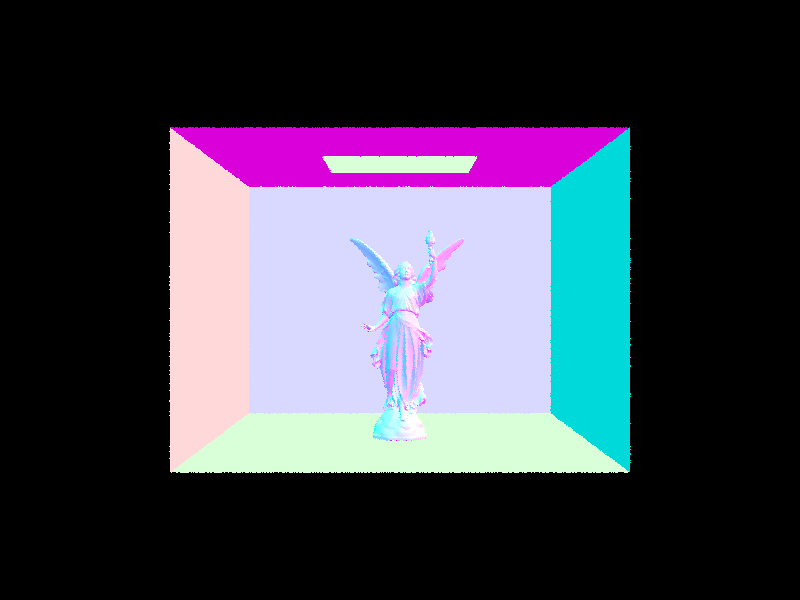
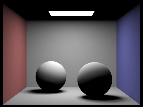
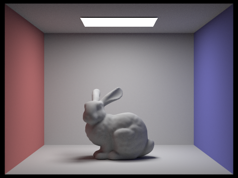
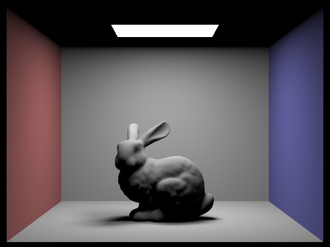
The direct illumination is significantly darker than the indirect illumination. The reason is that the direct illumination only considers the direct light from the light source, while the indirect illumination considers the light from the light source and the light from the other objects in the scene. This can be seen in the ceiling, where the direct illumination is completely black because it only allow light to bounce once, while the indirect one is not.

|

|

|

|

|
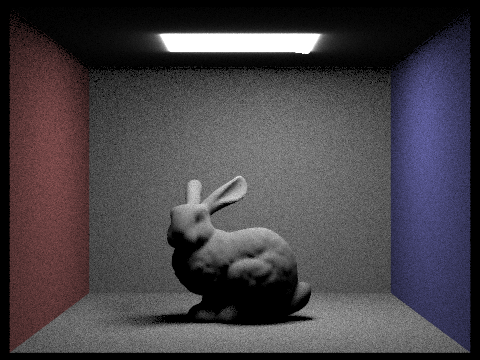
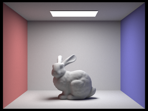
When max_ray_depth = 0, it works just the same as the direct illumination because every call to at_least_one_bounce_radiance will call one_bounce_radiance(r, isect) on the output vector and return(depth >= max_ray_depth). So it look exactly the same with direct lighting for the previous part. For max_ray_depth >= 1, it almost works as "two bounces" because it's likely to call one_bounce_radiance twice before returns.(if the russain roulette does not terminate). However, CBbunny is a smooth object with limited primitives and there is no other object in the scene, we can estimate that the ray.depth will not grow too large before it renders a decent image. As for max_ray_depth = 2,3,4,100, they look exactly the same with max_ray_depth = 1, which also proves that simplicity of this scene.
|
|
|
|

|

|

|
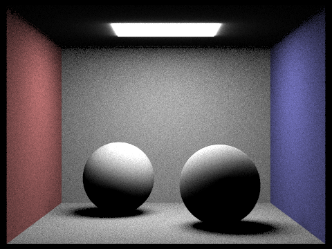
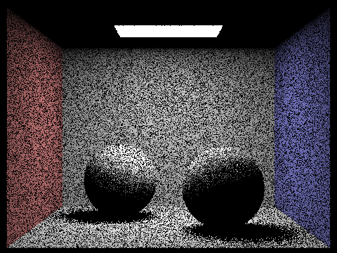
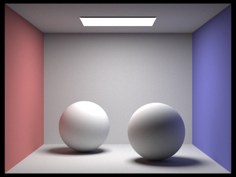
The images show that the number of sample per pixel is directly proportional to the quality of the image and inversely proportional to the rendering time. The reasons behind could be the light rays are undersampled. If we only have one sample per pixel, the sampling result might not fit the monte carlo integral very well. As the number of samples increases, it follows the Law of large numbers and the sampling result will converge to the integral if a proper PDF was used. However, the rendering time increases significantly as the number of samples increases. A sweat spot is between 512 to 1024 samples per pixel.
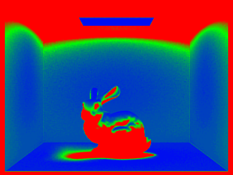
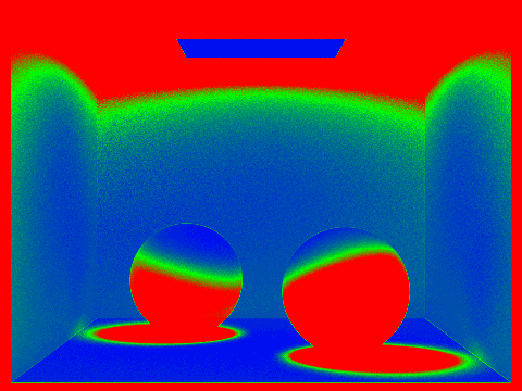
Adaptive sampling accelerates the rendering process by concentrating the samples in the more difficult parts of the image(I is big). When I converges, we think we can stop wasting more computational resources on this pixel and move on to the next. Adaptive sampling does a better job in eliminating the noise than fixed sampling.
Our implementation: Iterate through all the camera rays, and before anything has been done, we check whether a pixel has converged every samplesPerBatch pixels, if it has, we check if I is less than miu * max_tolerance, and if it is, we stop wasting more computational resources and move on to the next.
Otherwise, we treat it like a "regular" sample and update our result vectors accordingly.
|
|
|
|